Applications
Table of Contents
1 Applications
1.1 Mathematics
Trigonometric Degree Functions
deg2rad deg = deg*pi/180.0  -- convert degrees to radians
rad2deg rad = rad*180.0/pi  -- convert radians to degrees

sind = sin . deg2rad
cosd = cos . deg2rad
tand = tan . deg2rad
atand = rad2deg . atan
atan2d y x = rad2deg (atan2 y x )
Example:
> map rad2deg [pi/6, pi/4, pi/3, pi/2, pi]
[29.999999999999996,45.0,59.99999999999999,90.0,180.0]
>
>

> map sind [30.0, 45.0, 60.0, 90.0, 180.0 ]
[0.49999999999999994,0.7071067811865475,0.8660254037844386,1.0,1.2246063538223773e-16]
>
1.2 Piecewise Functions
Implement the following functions in Haskell
       /  0.10    if 0.0      <= x <= 7150.0
       |  0.15    if 7150.0   <  x <= 29050.0
       |  0.25    if 29050.0  <  x <= 70350.0
f1(x)= |  0.28    if 70350.0  <  x <= 146750.0
       |  0.33    if 146750.0 <  x <= 319100.0
       \  0.35    if 139100.0 <  x < +infinitum


       /  x^2 - 1  if x < 0
f2(x) = |  x   - 1  if 0 <= x < 4
       \  3        if x > 4
import Graphics.Gnuplot.Simple

(|>) x f = f x
(|>>) x f = map f x

pairs xs = zip xs (tail xs)

infp =    1.0e30  -- Plus Infinite
infm = (-1.0e30)  -- Minus Infinite

inInterval x (p1, p2) = (fst p1) < x && x <= (fst p2)

piecewiseFactory intervalTable x = f x
    where
    f =  filter (inInterval x) (pairs intervalTable)
        |> head
        |> fst
        |> snd

arange start stop step = [start,(start+step)..(stop-step)]

plotFxs f xs  = do
    let ys = map f xs
    plotList [] (zip xs ys)


f1_table =
    [
    (0.0,        const 0.10),
    (7150.0,     const 0.15),
    (29050.0,    const 0.25),
    (70350.0,    const 0.28),
    (146750.0,   const 0.33),
    (319100.0,   const 0.35),
    (1.0e30,     const 0.35)
    ]

f2_table = [
    (infm,  \x -> x**2 - 1), --  if -∞ < x <= 0  -> x^2 - 1
    (0.0,   \x -> x - 1.0 ), --  if 0  < x <= 4  -> x   - 1
    (4.0,   \x -> 3.0),      --  if 4  < x <= +∞ -> 3.0
    (infp,  \x -> 3.0 )
    ]

f1 = piecewiseFactory f1_table
f2 = piecewiseFactory f2_table
> plotFxs f1 $ arange (1.0) 400000 1000.0
!f1 chart
> plotFxs f2 $ arange (-4) 4 0.01
!f2 chart
1.3 Numerical Methods
1.3.1 Polynomial
Polynomial evaluation by the horner method.
polyval :: Fractional a => [a] -> a -> a
polyval coeffs x = foldr (\b c -> b + x*c) 0 coeffs

polyderv :: Fractional a => [a] -> [a]
polyderv coeffs = zipWith (*) (map fromIntegral [1..n]) (tail coeffs )
    where
    n = (length coeffs) - 1
Example:
Reference: http://www.math10.com/en/algebra/horner.html

f(x) = a0 + a1x + a2x2 + a3x3 + a4x4 + a5x5
f(x0) = a0 + x0(a1 + x0(a2 + x0(a3 + x0(a4 + a5x0))))

Example: Evaluate the polynomial
    f(x)  =  1x4 + 3x3 + 5x2 + 7x + 9 at x = 2
    df(x) =  3x3 + 6x2 + 10x +  7
> let coeffs  = [9.0, 7.0, 5.0, 3.0, 1.0]
> let f  = polyval  coeffs

let df = polyval $  polyderv coeffs

> polyderv coeffs
[7.0,10.0,9.0,4.0]

> f 2
83.0

> df 2
95.0

> (\x -> 7 + 10*x + 9*x^2 + 4*x^3) 2
95
1.3.2 Numerical Derivate
derv dx f x = (f(x+dx) - f(x))/dx

f x = 2*x**2 - 2*x
df = derv 1e-5 f

*Main> map f [2, 3, 4, 5]
[4.0,12.0,24.0,40.0]
*Main>

*Main> let df = derv 1e-5 f
*Main>
*Main> map df  [2, 3, 4, 5]
[6.000020000040961,10.000019999978349,14.000019999116374,18.000019998964945]
*Main>

*Main> let dfx x = 4*x - 2
*Main> map dfx [2, 3, 4, 5]
[6,10,14,18]
1.3.3 Nonlinear Equation - Root-finding
See also:
Bisection Method
bisection_iterator :: (Floating a, Floating a1, Ord a1) => (a -> a1) -> [a] -> [a]
bisection_iterator f guesslist = newguess
    where
    a =  guesslist !! 0
    b =  guesslist !! 1
    c = (a+b)/2.0
    p = f(a)*f(c)
    newguess = (\p -> if p < 0.0 then [a, c] else [c, b] ) p


bisectionSolver eps itmax f x1 x2 = (root, error, iterations)
    where

    bisection_error xlist = abs(f $ xlist !! 1)
    check_error xlist = bisection_error xlist > eps

    iterator = bisection_iterator  f

    rootlist = [x1, x2] |> iterate iterator |> takeWhile check_error |> take itmax

    pair = last rootlist |> iterator
    root = last pair
    error = bisection_error pair

    iterations = length rootlist

*Main> let f x  =  exp(-x) -3*log(x)
*Main> bisectionSolver 1e-5 100 f 0.05 3
(1.1154509544372555,8.86237816760671e-6,19)
*Main>
Newton Raphson Method
{-
Newton-Raphson Method Iterator, builds an iterator function
from the function to be solved and its derivate.

-}
newton_iterator f df x = x - f(x)/df(x)

{---------------------------------------------------------------------
    newtonSolver(eps, itmax, f, df, guess)

    Solve equation using the Newton-Raphson Method.

    params:

        eps   :  Tolerance of the solver
        itmax :  Maximum number of iterations
        f     :  Function which the root will be computed
        df    :  Derivate of the function
        guess :  Initial guess

newtonSolver
  :: (Fractional t, Ord t) =>
     t -> Int -> (t -> t) -> (t -> t) -> t -> (t, t, Int)
-----------------------------------------------------------------------
-}
newtonSolver :: (Floating t, Ord t) => t -> Int -> (t -> t) -> (t -> t) -> t -> (t, t, Int)
newtonSolver eps itmax f df guess = (root, error, iterations)
    where
    check_root x = abs(f(x)) > eps
    iterator = newton_iterator f df   -- Builds the Newton Iterator
    generator = iterate $ iterator    -- Infinite List that will that holds the roots (Lazy Evaluation)

    rootlist = take itmax $ takeWhile check_root $ generator guess
    root = iterator $ last $ rootlist
    error = abs(f(root))
    iterations = length rootlist


square_root a | a > 0       = newtonSolver 1e-6 50 (\x -> x^2 -a) (\x -> 2*x) a
              | otherwise   = error ("The argument must be positive")

{-
    Solve f(x) = x^2 - 2 = 0

    The solution is sqrt(2)
-}
> let f x = x^2 - 2.0
>
> let df x = 2*x
>
> let df x = 2.0*x
>
> newtonSolver 1e-3 100 f df 5
(1.414470981367771,7.281571315052027e-4,4)
>
> newtonSolver 1e-3 100 f df 50
(1.4142150098491113,4.094082521888254e-6,8)
>
Secant Method
(|>) x f = f x
(|>>) x f = map f x

secant_iterator :: Floating t => (t -> t) -> [t] -> [t]
secant_iterator f guesslist = [x, xnext]
    where
    x =  guesslist !! 0
    x_ = guesslist !! 1
    xnext = x - f(x)*(x-x_)/(f(x) - f(x_))

secantSolver eps itmax f x1 x2 = (root, error, iterations)
    where

    secant_error xlist = abs(f $ xlist !! 1)
    check_error xlist = secant_error xlist > eps

    iterator = secant_iterator  f

    rootlist = [x1, x2] |> iterate iterator |> takeWhile check_error |> take itmax

    pair = last rootlist |> iterator
    root = last pair
    error = secant_error pair

    iterations = length rootlist

*Main> let f x = x^2 - 2.0
*Main> secantSolver  1e-4 20 f 2 3
(1.4142394822006472,7.331301515467459e-5,6)
*Main>
*Main> let f x = exp(x) - 3.0*x^2
*Main> secantSolver 1e-5 100 f (-2.0)  3.0
(-0.458964305393305,6.899607281729558e-6,24)
*Main>
1.3.4 Differential Equations
Euler Method
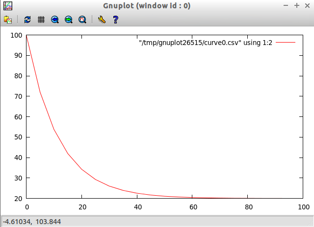
The task is to implement a routine of Euler's method and then to use it to solve the given example of Newton's cooling law with it for three different step sizes of 2 s, 5 s and 10 s and to compare with the analytical solution. The initial temperature T0 shall be 100 °C, the room temperature TR 20 °C, and the cooling constant k 0.07. The time interval to calculate shall be from 0 s to 100 s
From: http://rosettacode.org/wiki/Euler_method
Solve differential equation by the Euler's Method.

    T(t)
    ---- =  -k(T(t) - Tr)
     dt

    T(t) = Tr + k(T0(t) - Tr).exp(-k*t)
import Graphics.Gnuplot.Simple


eulerStep f step (x, y)= (xnew, ynew)
                    where
                    xnew = x + step
                    ynew = y + step * (f (x, y))

euler :: ((Double, Double) -> Double) -> Double -> Double -> Double -> Double -> [(Double, Double)]
euler f x0 xf y0 step = xypairs
                     where
                     iterator = iterate $ eulerStep f step
                     xypairs = takeWhile (\(x, y) -> x <= xf ) $ iterator (x0, y0)

> let dTemp k temp_r (t, temp) = -k*(temp - temp_r)

> euler (dTemp 0.07 20.0) 0.0 100.0 100.0 5.0
[(0.0,100.0),(5.0,72.0),(10.0,53.8),(15.0,41.97) \.\.\.
(100.0,20.01449963666907)]
>

let t_temp = euler (dTemp 0.07 20.0) 0.0 100.0 100.0 5.0

plotList [] t_temp
Runge Kutta RK4
See also: Runge Kutta Methods
import Graphics.Gnuplot.Simple

rk4Step f h (x, y) = (xnext, ynext)
                      where

                      k1 = f (x, y)
                      k2 = f (x+h/2, y+h/2*k1)
                      k3 = f (x+h/2, y+h/2*k2)
                      k4 = f (x+h,y+h*k3)

                      xnext = x + h
                      ynext = y + h/6*(k1+2*k2+2*k3+k4)

rk4 :: ((Double, Double) -> Double) -> Double -> Double -> Double -> Double -> [(Double, Double)]
rk4 f x0 xf y0 h = xypairs
                     where
                     iterator = iterate $ rk4Step f h
                     xypairs = takeWhile (\(x, y) -> x <= xf ) $ iterator (x0, y0)

> let dTemp k temp_r (t, temp) = -k*(temp - temp_r)
>
> let t_temp = rk4 (dTemp 0.07 20.0) 0.0 100.0 100.0 5.0
> plotList [] t_temp
>
1.4 Statistics and Time Series
1.4.1 Some Statistical Functions
Arithmetic Mean of a Sequence
mean lst = sum lst / fromIntegral (length lst)
Geometric Mean of Sequence
geomean lst = (product lst) ** 1/(fromIntegral (length lst))
Convert from decimal to percent
to_pct   lst = map (100.0 *) lst {- Decimal to percent -}
from_pct lst = map (/100.0)  lsd {- from Percent to Decimal -}
Lagged Difference of a time serie
- lagddif [xi] = [x_i+1 - x_i]
lagdiff lst = zipWith (-) (tail lst) lst
Growth of a Time Series
- growth [xi] = [(x_i+1 - x_i)/xi]
growth lst = zipWith (/) (lagdiff lst) lst
Percentual Growth
growthp = to_pct . growth
Standard Deviation and Variance of a Sequence
{- Standard Deviation-}
stdev values =  values   |>> (\x -> x -  mean values ) |>> (^2) |> mean |> sqrt

{- Standard Variance -}
stvar values = stdev values |> (^2)
Example: Investment Return
The annual prices of an Blue Chip company are given below, find the percent growth rate at the end of each year and the CAGR Compound annual growth rate.
year    0    1     2     3     4     5
price  16.06 23.83 33.13 50.26 46.97 39.89
Solution:
> let (|>) x f = f x
> let (|>>) x f = map f x
>
> let cagr prices = (growthp prices |>> (+100) |> geomean ) - 100
>
> let prices = [16.06, 23.83, 33.13, 50.26, 46.97, 39.89 ]
>
> {- Percent Returns -}
> let returns = growthp prices
>
> returns
[48.38107098381071,39.02643726395302,51.705402958044054,-6.545961002785513,-15.073451139024908]
>

> let annual_cagr = cagr prices
> annual_cagr
19.956476057259906
>
1.4.2 Monte Carlo Simulation Coin Toss
The simplest such situation must be the tossing of a coin. Any individual event will result in the coin falling with one side or the other uppermost (heads or tails). However, common sense tells us that, if we tossed it a very large number of times, the total number of heads and tails should become increasingly similar. For a greater number of tosses the percentage of heads or tails will be next to 50% in a non-biased coin. Credits: Monte Carlo Simulation - Tossing a Coin

File: coinSimulator.hs
import System.Random
import Control.Monad (replicateM)

{-
    0 - tails
    1 - means head

-}

flipCoin :: IO Integer
flipCoin = randomRIO (0, 1)

flipCoinNtimes n = replicateM n flipCoin

frequency elem alist = length $ filter (==elem) alist

relativeFreq :: Integer -> [Integer] -> Double
relativeFreq elem alist =
    fromIntegral (frequency elem alist) / fromIntegral (length alist)

simulateCoinToss ntimes =  do
    series <- (flipCoinNtimes  ntimes)
    let counts = map (flip frequency series)   [0, 1]
    let freqs = map (flip relativeFreq series) [0, 1]
    return (freqs, counts)

showSimulation ntimes = do
    result <- simulateCoinToss ntimes
    let p_tails = (fst result) !! 0
    let p_heads = (fst result) !! 1

    let n_tails = (snd result) !! 0
    let n_heads = (snd result) !! 1

    let tosses = n_tails + n_heads
    let p_error = abs(p_tails - p_heads)

    putStrLn $ "Number of tosses : " ++ show(tosses)
    putStrLn $ "The number of tails is : " ++ show(n_tails)
    putStrLn $ "The number of heads is : " ++ show(n_heads)
    putStrLn $ "The % of tails is : " ++ show(100.0*p_tails)
    putStrLn $ "The % of heads is :" ++ show(100.0*p_heads)
    putStrLn $ "The %erro is : "  ++ show(100*p_error)
    putStrLn "\n-------------------------------------"
> :r
[1 of 1] Compiling Main             ( coinSimulator.hs, interpreted )
Ok, modules loaded: Main.
>

> :t simulateCoinToss
simulateCoinToss :: Int -> IO ([Double], [Int])
>

> :t showSimulation
showSimulation :: Int -> IO ()
>


> simulateCoinToss 30
([0.5666666666666667,0.43333333333333335],[17,13])
>
> simulateCoinToss 50
([0.56,0.44],[28,22])
>
> simulateCoinToss 100
([0.46,0.54],[46,54])
>
> simulateCoinToss 1000
([0.491,0.509],[491,509])
>

> mapM_ showSimulation [1000, 10000, 100000, 1000000]
Number of tosses : 1000
The number of tails is : 492
The number of heads is : 508
The % of tails is : 49.2
The % of heads is :50.8
The %erro is : 1.6000000000000014

-------------------------------------
Number of tosses : 10000
The number of tails is : 4999
The number of heads is : 5001
The % of tails is : 49.99
The % of heads is :50.01
The %erro is : 1.9999999999997797e-2

-------------------------------------
Number of tosses : 100000
The number of tails is : 49810
The number of heads is : 50190
The % of tails is : 49.81
The % of heads is :50.19
The %erro is : 0.38000000000000256

-------------------------------------
Number of tosses : 1000000
The number of tails is : 499878
The number of heads is : 500122
The % of tails is : 49.9878
The % of heads is :50.01219999999999
The %erro is : 2.4399999999996647e-2

-------------------------------------
1.5 Vectors
Dot Product of Two Vectors / Scalar Product
- v1.v2 = (x1, y1, z1) . (x2, y2, z2) = x1.y1 + y1.y2 + z2.z1
- v1.v2 = Σai.bi
> let dotp v1 v2 = sum ( zipWith (*) v1 v2 )   - With Parenthesis
> let dotp v1 v2 = sum $ zipWith (*) v1 v2     - Without Parenthesis with $ operator

> dotp [1.23, 33.44, 22.23, 40] [23, 10, 44, 12]
1820.81
Norm of a Vector
- norm = sqrt( Σxi^2)
> let norm vector = (sqrt . sum) (map (\x -> x^2) vector)

> norm [1, 2, 3, 4, 5]
7.416198487095663

-- Vector norm in multiple line statements in GHCI interactive shell

> :{
| let {
|      norm2 vec =  sqrt(sum_squares)
|      where
|      sum_squares = sum(map square vec)
|      square x = x*x
|      }
| :}
>
> norm2 [1, 2, 3, 4, 5]
7.416198487095663
>
Linspace and Range Matlab Function
linspace d1 d2 n = [d1 + i*step | i <- [0..n-1] ]
    where
    step = (d2 - d1)/(n-1)


range start stop step =  [start + i*step | i <- [0..n] ]
    where
    n = floor((stop - start)/step)
1.6 Tax Brackets
Progressive Income Tax Calculation
Credits: Ayend - Tax Challange
The following table is the current tax rates in Israel:
                        Tax Rate
Up      to 5,070        10%
5,071   up to 8,660     14%
8,661   up to 14,070    23%
14,071  up to 21,240    30%
21,241  up to 40,230    33%
Higher  than 40,230     45%
Here are some example answers:
5,000 –> 500
5,800 –> 609.2
9,000 –> 1087.8
15,000 –> 2532.9
50,000 –> 15,068.1
This problem is a bit tricky because the tax rate doesn’t apply to the whole sum, only to the part that is within the current rate.
A progressive tax system is a way to calculate a tax for a given price using brackets each taxed separately using its rate. The french tax on revenues is a good example of a progressive tax system.
To calculate his taxation, John will have to do this calculation
(see figure on left):

= (10,000 x 0.105) + (35,000 x 0.256) + (5,000 x 0.4)
= 1,050 + 8,960 + 2,000
= 12,010

John will have to pay $ 12,010

If John revenues was below some bracket definition (take $ 25,000 for
example), only the last bracket containing the remaining amount to be
taxed is applied :

= (10,000 x 0.105) + (15,000 x 0.256)

Here nothing is taxed in the last bracket range at rate 40.
Solution:
(|>) x f = f x
(|>>) x f = map f x
joinf functions element = map ($ element) functions

-- Infinite number
above = 1e30

pairs xs = zip xs (tail xs)

{-
    Tax rate function - Calculates the net tax rate in %

    taxrate = 100 *  tax / (gross revenue)

-}
taxrate taxfunction income = 100.0*(taxfunction income)/income

progressivetax :: [[Double]] -> Double -> Double
progressivetax taxtable income = amount
            where
            rates = taxtable |>> (!!1) |>> (/100.0)  |> tail
            levels = taxtable |>> (!!0)
            table = zip3 levels (tail levels) rates
            amount = table |>> frow income |> takeWhile (>0) |> sum

            frow x (xlow, xhigh, rate) | x > xhigh = (xhigh-xlow)*rate
                                       | otherwise = (x-xlow)*rate
taxsearch taxtable value = result
        where
        rows = takeWhile (\row -> fst row !! 0 <= value) (pairs taxtable)
        result = case rows of
                    [] -> taxtable !! 0
                    xs -> snd $ last rows

{-
   This is useful for Brazil income tax calculation

  [(Gross Salary  – Deduction - Social Security ) • Aliquot – Deduction] = IRRF
  [(Salário Bruto – Dependentes – INSS) • Alíquota – Dedução] =

-}
incometax taxtable income  = amount--(tax, aliquot, discount)
                where

                row = taxsearch taxtable income
                aliquot = row !! 1
                discount = row !! 2
                amount = income*(aliquot/100.0) - discount

{- Progressive Tax System -}
israeltaxbrackets = [
    [0,          0],
    [ 5070.0, 10.0],
    [ 8660.0, 14.0],
    [14070.0, 23.0],
    [21240.0, 30.0],
    [40230.0, 33.0],
    [above  , 45.0]
    ]

taxOfIsrael     = progressivetax israeltaxbrackets
taxRateOfIsrael = taxrate taxOfIsrael

braziltaxbrackets = [
    [1787.77,    0,   0.00],
    [2679.29,  7.5, 134.48],
    [3572.43, 15.0, 335.03],
    [4463.81, 22.5, 602.96],
    [above,    27.5, 826.15]
   ]


taxOfBrazil = incometax braziltaxbrackets
taxRateOfBrazil = taxrate  taxOfBrazil


{-
    Unit test of a function of numerical input and output.

    input       - Unit test case values             [t1, t2, t2, e5]
    expected    - Expected value of each test case  [e1, e2, e3, e4]
    tol         - Tolerance 1e-3 typical value
    f           - Function:                         error_i = abs(e_i-t_i)

    Returns true if in all test cases  error_i < tol
-}
testCaseNumeric :: (Num a, Ord a) => [a1] -> [a] -> a -> (a1 -> a) -> Bool
testCaseNumeric input expected tol f = all (\t -> t && True) ( zipWith (\x y -> abs(x-y) < tol) (map f input) expected )

testIsraelTaxes = testCaseNumeric
    [5000, 5800, 9000, 15000, 50000]
    [500.0,609.2,1087.8,2532.9,15068.1]
    1e-3 taxOfIsrael

> testIsraelTaxes
True
>
>
> taxOfIsrael 5000
500.0
> taxOfIsrael 5800
609.2
> taxOfIsrael 1087.8
108.78
> taxOfIsrael 15000.0
2532.9
> taxOfIsrael 50000.0
15068.1
>
> taxRateOfIsrael 5000
10.0
> taxRateOfIsrael 5800
10.50344827586207
> taxRateOfIsrael 15000
16.886
> taxRateOfIsrael 50000
30.1362
Sources:
1.7 Small DSL Domain Specific Language
Simple DSL for describing cups of Starbucks coffee and computing prices (in dollars). Example taken from: http://www.fssnip.net/9w
starbuck_dsl.hs
data Size  = Tall | Grande | Venti
            deriving (Eq, Enum, Read, Show, Ord)

data Drink = Latte | Cappuccino | Mocha | Americano
            deriving (Eq, Enum, Read, Show, Ord)

data Extra = Shot | Syrup
            deriving (Eq, Enum, Read, Show, Ord)

data Cup = Cup {
                cupDrink :: Drink,
                cupSize  :: Size,
                cupExtra :: [Extra]
               }
               deriving(Eq, Show, Read)

{-
 -                  Table in the format:
 -                 -------------------
 -                  tall, grande, venti
 -    Latte         p00   p01     p02
 -    Cappuccino    p10   p11     p12
 -    Mocha         p20   p21     p22
 -    Amaericano    p30   p31     p32
 -}

table = [
    [2.69, 3.19, 3.49],
    [2.69, 3.19, 3.49],
    [2.99, 3.49, 3.79],
    [1.89, 2.19, 2.59]
    ]


extraPrice :: Extra -> Double
extraPrice Syrup = 0.59
extraPrice Shot  = 0.39

priceOfcup cup =  baseprice + extraprice
            where
            drinkrow = table !!  fromEnum  (cupDrink cup)
            baseprice   = drinkrow !!  fromEnum  (cupSize cup)
            extraprice = sum $ map extraPrice (cupExtra cup)


{- Constructor of Cup -}
cupOf drink size extra = Cup {
                             cupSize = size,
                             cupDrink = drink,
                             cupExtra = extra}

drink_options = [ Latte, Cappuccino, Mocha, Americano]
size_options  = [ Tall, Grande, Venti]
extra_options = [[], [Shot], [Syrup], [Shot, Syrup]]

cup_combinations =
            [ cupOf drink size extra | drink <- drink_options, size <- size_options, extra <- extra_options]
Example:
> :load starbucks_dsl.hs
[1 of 1] Compiling Main             ( starbucks_dsl.hs, interpreted )
Ok, modules loaded: Main.
>
>

> let myCup = cupOf Latte Venti [Syrup]
> let price = priceOfcup myCup
> myCup
Cup {cupDrink = Latte, cupSize = Venti, cupExtra = [Syrup]}
> price
4.08
>

> priceOfcup (cupOf Cappuccino Tall [Syrup, Shot])
3.67
>

> let cups = [ cupOf Americano Venti extra |  extra <- extra_options]
> cups
[Cup {cupDrink = Americano, cupSize = Venti, cupExtra = []},
Cup {cupDrink = Americano, cupSize = Venti, cupExtra = [Shot]},
Cup {cupDrink = Americano, cupSize = Venti, cupExtra = [Syrup]},
Cup {cupDrink = Americano, cupSize = Venti, cupExtra = [Shot,Syrup]}]
>

> let prices = map priceOfcup cups
> prices
[2.59,2.98,3.1799999999999997,3.57]
>

> let cupPrices = zip cups prices
> cupPrices
[(Cup {cupDrink = Americano, cupSize = Venti, cupExtra = []},2.59),
(Cup {cupDrink = Americano, cupSize = Venti, cupExtra = [Shot]},2.98),
(Cup {cupDrink = Americano, cupSize = Venti, cupExtra = [Syrup]},3.1799999999999997),
(Cup {cupDrink = Americano, cupSize = Venti, cupExtra = [Shot,Syrup]},3.57)]
>